It All Adds Up: Mathematics on the FE Electrical Exam

For those looking to take the Fundamentals of Engineering (FE) Electrical Engineering (EE) exam, we will delve into various concepts and components of mathematics, including:

 

1. Algebra and trigonometry

2. Complex numbers

3. Discrete mathematics

4. Analytic geometry

5. Calculus

6. Ordinary differential equation

7. Matrix Operation

8. Vector Analysis

Please note that the materials presented here are an overview. We encourage you to explore further resources if you wish to learn more about any particular topic.

In this blog,

1. Algebra and Trigonometry

    a. Algebra

    b. Trignometry

2. Complex Numbers

    a. Rectangular Form

    b. Polar Form

3. Discrete Mathematics

4. Analytic Geometry

    a. Slope of Equation

    b. Conic Section

Algebra and Trigonometry

A. Algebra

Algebra serves as an essential cornerstone in the realm of engineering. Nearly all analytical assessments in engineering require the use of algebraic equations. To adequately equip oneself for the FE Electrical exam, it is paramount to possess the proficiency to adeptly manipulate elementary algebraic equations, enabling the subsequent determination of solutions. This segment showcases illustrative instances of equation manipulations for comprehensive comprehension.

 

B. Trigonometry

Within the “Mathematic” section of the FE Reference Handbook, one can find a comprehensive compilation of essential trigonometric relations.

A notable use of trigonometry is analyzing the behavior of right triangles (Figure 1).

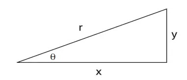
Figure 1

sin θ = y/r; cos θ = x/r; tan θ = y/x; cot θ = x/y; csc θ = r/y

sec θ = r/x

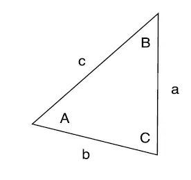
However, for non-right triangles, we cannot apply the above trigonometric relation to solve for the unknown values. Using the law of sines and cosines, all unknowns of a triangle can be characterized (Figure 2).

Figure 2

The law of sines is depicted below:

 a/sin A = b/sin B  = c/sin C

The law of cosines is depicted below:

a²= b²+ c² – 2bc cos A 

b²= a²+ c² – 2ac cos A
 

c²= a²+ b² – 2ab cos C

Complex Numbers

Complex numbers are a mathematical characterization equation that combines both a real part and an imaginary part (Electronics Tutorials, n.d.). It is typically written in the form

y = a + jb (1)

Where,

 a = real component

b = imaginary component, and j is the imaginary variable with the unit of √(-1). 

Complex numbers allow for the representation and manipulation of quantities that involve both real and imaginary components, extending the number system beyond the realm of real numbers.

There are two forms that the complex numbers can be represented: rectangular form or polar form (Electronics Tutorials, n.d.).

 

A. Rectangular Form

In the context of complex numbers, the rectangular form refers to a way of representing a complex number using its real and imaginary parts.

y = a + jb

B. Polar Form

In complex numbers, the polar form represents a way of expressing a complex number using its magnitude (or modulus) and argument (or angle). A complex number in polar form is written.

y = r(cos cos θ + jsin sin θ)=  z∠θ

To convert the complex number from rectangular form  to polar form, we can use the following formulas:

z = √(a²+b² )

θ = (b/a)  (in degree)

Conversely, to convert a complex number from polar form to rectangular form, we can use the following formulas:

a = r × cos cos θ 

b = r × sin sin θ 

Complex numbers can be added, subtracted, multiplied, and divided. Let’s say we have these 2 complex numbers:

A = 2+3j

B = -1+4j

Given the above values, complex numbers can be added and subtracted in rectangular form:

1. A + B = 2 + (-1) +3j  +4j  = 1 + 7j

2. A – B = 2 – (-1) + 3j - 4j = 3 - j

While, multiplying and dividing is performed in the polar form:

1. Convert the complex number A and B into polar form

a. For A: z = √(2²+3² ) = 3.6056 and θ = (3/2) = 56.31 deg . So, A = 3.6056 ∠56.31deg.

b. For B: z = √(〖(-1)〗²+4² ) = 4.123 and θ = (4/(-1)) =104.04 deg . So, B = 4.123∠104.04deg.

2. When A x B:

A x B = 3.6056∠56.31deg × 4.123∠104.04deg = = 3.6056*4.123∠(56.31+104.04) =14.87∠160.35deg

3. When A / B: 

A / B = (3.6056∠56.31) / (4.123∠104.04) = 3.6056/4.123∠(56.31-104.04) = 0.87∠-47.73deg. 

Discrete Mathematics

Discrete mathematics is a branch of mathematics that deals with mathematical structures and techniques focused on countable or finite sets. It encompasses topics such as graph theory, combinatorics, set theory, logic, and algorithms, which are instrumental in solving problems involving discrete structures and countable sets (Hayes et al., n.d.).

Set theory is key within discrete mathematics, it is the study of collections of objects. Set operations, such as union (∪), intersection (∩) , and complement (') are fundamental in set theory (Hayes et al., n.d.).

Example:

Suppose we have two sets A = {1, 2, 3} and B = {2, 3, 4}. The union of A and B (A ∪ B) is then represented as {1, 2, 3, 4}, and all the distinct elements from both sets are outputted. The intersection of sets A and B (A ∩ B) is then represented as {2, 3}, and all the common elements between the sets are outputted. The complement of set A (A') is the set of all elements not present in A.

For further information about discrete mathematics, you can visit this website to explore more!

Analytic Geometry

Analytic geometry, also known as coordinate geometry, is a branch of mathematics that combines algebraic techniques with geometric concepts. It involves studying geometric figures and relationships using algebraic equations and coordinates.

In analytic geometry, points, lines, curves, and other geometric objects are shown using coordinates in a coordinate system: Cartesian coordinate system. The Cartesian coordinate system consists of two perpendicular lines called the x-axis and y-axis, intersecting at a point called the origin (Nykamp, n.d.). Each point in the plane is uniquely identified by its x-coordinate (horizontal position) and y-coordinate (vertical position).

A. Slope of Equation

The x-y plane serves as a two-dimensional coordinate system that represents pairs of values (x, y). These pairs, known as ordered pairs, are referred to as points. A line can be defined by two points. The equation of a line can be expressed in the slope-intercept form, which is given by:

y = mx+b

Where,

m is the slope of the line

 b = y intercept, where b is the value of y when  x = 0;

The slope between two points can be found by:

m=(y₂-y₁)/(x₂-x₁ ) 

By rearranging the slope equation, it becomes possible to calculate the value of "b" using any point that is provided on the line.

b = y - mx

Example:

Given two points (10, 20) and (-30, -40). Find the line equation

1. m = (-40-20) / (-30-10) = (-60) / (-40) = 1.5

2. We will pick the first point (10, 20) to solve for b

b = y - mx = 20 – (1.5)(10) = 5

Therefore,  y =1.5x + 5

B. Conic Section

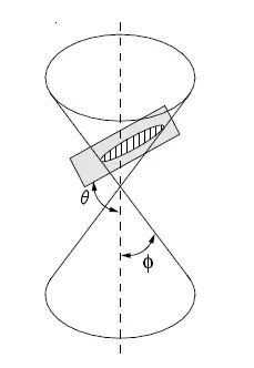
Conic sections are an important class of equations involving two variables. They encompass four types: parabolas, ellipses, hyperbolas, and circles. The term "conic section" originates from the concept of intersecting a cone with a plane in different configurations.

Figure 3

When a plane intersects a three-dimensional double right circular cone at various positions and angles, it gives rise to conic sections (refer to Figure 3). The equation describing the resulting conic section depends on the characteristics of the cone, specifically the angle between the cone's side and its axis (ϕ), as well as the angle between the intersecting plane and the cone's axis (θ). The relationship between the plane and the cone is quantified by the eccentricity (e) (Strang & Herman, 2022).

In the FE exam, the problems pertaining to this section are presented in a straightforward manner. One can employ the provided equations and relationships to determine the unknown values based on the specific type of conic section involved. It is crucial to thoroughly read and comprehend the problem statement in order to correctly identify and utilize the appropriate equation.

Conclusion

This is a lot of information to sort through on first reading, so please take the time to reread and practice the problems on your own. We will finish the other half in the second part of this blog. Are you interested in a comprehensive exam review course that will cover the topics of this blog and more? Check out School of PE’s FE Electrical exam review courses now.

References

Electronics Tutorials. (n.d.). Complex Numbers and Phasors in Polar and Rectangular Form. Electronics Tutorials. Retrieved July 6, 2023, from https://www.electronics-tutorials.ws/accircuits/complex-numbers.html

Hayes, A., Parvej, M. R., Vee, H. Z., Nelson, A., & Khim, J. (n.d.). Discrete Mathematics. Brilliant. Retrieved July 5, 2023, from https://brilliant.org/wiki/discrete-mathematics/

Nykamp, D. Q. (n.d.). Cartesian coordinates. Math Insight. Retrieved July 6, 2023, from https://mathinsight.org/cartesian_coordinates

Strang, G., & Herman, E. '. (2022, September 7). 11.5: Conic Sections. Mathematics LibreTexts. Retrieved July 6, 2023, from https://math.libretexts.org/Bookshelves/Calculus/Calculus_(OpenStax)/11%3A_Parametric_Equations_and_Polar_Coordinates/11.05%3A_Conic_Sections

About the Author: Khoa Tran

Khoa Tran is an electrical engineer working at the Los Angeles Department of Water and Power and is currently pursuing his master's in electrical Power from the University of Southern California. He is fluent in both Vietnamese and English and is interested in outdoor activities and exploring new things.