


 FE Courses
 PE Courses
 SE Courses
 Continuing Education
 Pmp Courses
 Corportate Training
Welcome back to our introduction to mathematics! Continuing from where we left off, we will explore calculus, ordinary differential equations, linear algebra, and vector analysis.
Calculus
A. Derivative
The derivative of a function determines the immediate rate of change. Visually, it represents the slope depicted by the original function.
The basic rules of derivative include: derivative of sum, derivative of product, and derivative of quotient. The derivative of the sum is straightforward; you just need to take the derivative of each term. When it comes to multiplication, we have the product rule (Eqn 1).
dy/dx = u dv/dx + v du/dx (1)
And the quotient rule (Eqn 2) to use for the division.
dy/dx = (v du/dx-u dv/dx)/v2 (2)
The chain rule is a formula for finding the derivative of the composite of 2 functions. The chain rule helps to differentiate composite functions (find the derivative of a composite function). Generally, there is an “inside function” and an “outside function” that are both differentiable (Orloff, 2023).
(d[(f(u)])/dx = (d[f(u)]) /du du/dx (3) or
f(g(x))' = f'(g(x))*g'(x) (4)
B. Integral
The integral, or antiderivative, permits the calculation of the area under a curve or between curves.
Basic techniques for integrals:
1. Look for ways to simplify the integral with algebra before integrating.
2. Refer to the indefinite integrals on page 49 of the FE reference handbook.
3. Plug in the initial value and solve for the constant.
When integrals are more complicated, other methods of integration that can be used are:
1. Integration by Parts
2. Substitution
I. Integration by Parts
Integration by parts evaluates integrals of products of functions. It is based on the product rule of differentiation, which states that the derivative of the product of two functions is equal to the first function times the derivative of the second function, plus the second function times the derivative of the first function (Strang & Herman, 2022).
∫ u dv = uv - ∫ v du (5)
II. Substitution
U-substitution, also known as “Integration by Substitution” or “The Reverse Chain Rule”, is a method to simplify and evaluate integrals by use of substitution. To begin, ensure the integral is written in its standard form:
∫ f(g(x))g'(x) dx, (6)
Then substitute in the variable “u.” ∫ f(u) du (7)
This replacement reduces a complicated expression into a simpler form that can be more easily evaluated.
The U-substitution is as follows (Mathematics LibreTexts, 2020):
1. Identify an expression within the integrand which appears to be a derivative of some function.
2. Choose a new variable "u" to represent the chosen expression. Do not forget to include the corresponding differential "du" to the derivative of "u" with respect to the original.
3. Rewrite the entire integral and substituting in the new variable "u", effectively replacing the complicated expression with "u".
4. Evaluate the new integral with respect to "u" using standard integration techniques, which may involve simpler rules or known integral formulas.
5. Finally, substitute the original variable back into the result by replacing "u" with the expression chosen in step 2.
Ordinary Differential Equation
A differential equation is a mathematical equation that involves an unknown function and its derivatives. It describes the relationship between the function and its rates of change. In essence, a differential equation expresses how the function's behavior changes based on its current state and the values of its derivatives (Herman, 2018).
The FE Reference Handbook provides a comprehensive collection of equation forms necessary for solving first-order and second-order homogeneous differential equations. These invaluable resources can be found on pages 52 and 53 of the handbook. To further enhance your understanding and proficiency, you can explore additional illustrative examples by following this link.
Matrix Operations
Matrix operations refer to various mathematical operations performed on matrices, which are rectangular arrays of numbers. Matrix operations allow for the manipulation, combination, and transformation of matrices, enabling the analysis of systems of linear equations, geometric transformations, and other mathematical applications.
In this section, I will not go too in-depth since you can use a calculator to manipulate matrices in the FE exam. You can visit this link to do matrix multiplication and this link on how to find the inverse and adjoint of a matrix.
Vector Analysis
A vector embodies the essence of a physical property, possessing not only its size but also its orientation. Its portrayal in three-dimensional space is accomplished by its x, y, and z constituents (Corral, 2023), often denoted as
F = ax i + ay j + az k (8)
where:
ax, ay, az are the component magnitudes in the x, y, and z directions.
i,j,k are the unit vectors establishing coordinate direction for the vector.
The magnitude of vector F is calculated as:
F = √(〖ax〗2 +〖ay〗2 +〖az〗2 ) (9)
A wide array of operations can be performed with vectors, benefiting from their linear nature, which ensures clear and precise outcomes.
Among the operations involving vectors are addition, subtraction, and multiplication, which are essentially akin to basic algebraic procedures. Scalar multiplication entails the multiplication of a scalar by a vector. The dot product, on the other hand, determines the angle between two vectors.
A. Vector Addition and Subtraction
Vector addition is the process of combining two or more vectors to obtain a resultant vector. Vector subtraction involves a reversal in direction, achieved by adding negative vectors. A negative vector possesses an equal magnitude to that of a positive addition vector but points in the opposite direction.
A ± B = (ax ± bx)i + (ay ± by)j + (az ± bz)k (10)
B. Vector Dot Product
Also known as the scalar product, it is the operation that yields a scalar value by taking the sum of the products of the corresponding components of two vectors (Corral, 2023).
A∙B = (ax bx) + (ay by) + (az bz) (11) (this produces a scalar)
or
A∙B = |A||B|cosθ = B∙A (12) (this produces the projection)
By rearranging the equation, the dot product can be utilized to ascertain the angle between two vectors, as illustrated in Figure 1. This rearrangement involves employing the cosine of the angle equation for the dot product.
cos θ = (A∙B) / |A||B| (13)
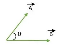
Figure 1
C. Vector Cross Product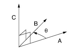.webp)
 The sense of A X B is determined by the right-hand rule:
The cross product yields a third vector, adhering to the principles of the right-hand rule, which resides orthogonal to the plane encompassing the initial two vectors. As vector A gracefully intertwines with vector B, it imparts the orientation of vector C, unfolding a trajectory perpendicular to their shared plane (Figure 2) (Corral, 2023).
Figure 2
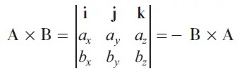
The cross product is illustrated as a 3x3 matrix:
A × B = |A||B|n sin θ (14)
Where,
n is the unit vector perpendicular to the plane of A and B.
Conclusion
Although this blog provides an overview of mathematical topics found on the FE Electrical exam, you can find a more thorough explanation in School of PE’s FE Electrical exam review course. Learn more or register for a course now!
No comments :
Post a Comment