Unraveling the Impact: How the Pandemic Affected FE Exam Candidates

In early 2020, the world was locked down due to a nightmarish virus: COVID-19. As the virus spread rapidly across the globe, it brought about significant disruptions across a multitude of sectors, including education. Among those heavily impacted were aspiring engineers preparing for the Fundamentals of Engineering (FE) exam, a critical milestone for their professional journey. This blog aims to dive deeper into the ways in which the pandemic affected all FE exam candidates, explore the challenges they faced, and highlight the remarkable resilience they displayed in adapting to these difficult circumstances.

In this Blog,

1.The Shift to Remote Learning: Challenges and Opportunities

2.Disrupted Study Routines: Maintaining Focus Amidst Chaos

3.Limited Access to Resources: Overcoming Obstacles

4.Canceled or Delayed Exams: Coping with Uncertainty

5. Emotional Toll and Mental Health Challenges: Nurturing Well-being

1. The Shift to Remote Learning: Challenges and Opportunities

When the pandemic struck, schools and universities were forced to lock up their doors, causing a rapid shift from traditional, in-person learning to remote education. For FE exam candidates, this meant embracing online lectures, virtual study groups, and digital resources as the new norm. While initially, this new digital environment offered plenty of conveniences, such as schedule flexibility and greater accessibility, it also came with a set of new challenges.

The abrupt shift to remote learning forced all candidates to adapt to a different learning style. Some individuals were able to thrive in the virtual environment, finding it more conducive to their own study habits. However, there were others who struggled to adapt, facing technical difficulties or struggling to maintain focus without the structure of a physical classroom.

Social distancing exasperated the issue, forbidding friends, colleagues, and all other established study groups from gathering personally. The lack of face-to-face interactions with peers and instructors also deprived candidates of valuable opportunities for immediate feedback and collaboration.

 

2. Disrupted Study Routines: Maintaining Focus Amidst Chaos

An effective study routine is fundamental for success in all exams, and the pandemic wreaked havoc on candidates' established study habits. Many found themselves engulfed by the many distractions found at home, making it incredibly challenging for many to maintain their concentration and discipline during their dedicated study sessions. The lines between personal and academic spaces blurred, increasing the likelihood of procrastinating and reducing productivity.

Additionally, the pandemic imposed additional responsibilities and greater stress on some candidates. For instance, those living with high-risk family members or roommates were required to become caretakers during the pandemic, drastically reducing any available study time. Others were faced with immense financial strain due to unexpected job losses or economic uncertainties, forcing them to put greater effort into searching and taking on more work alongside their exam preparations.

 

3. Limited Access to Resources: Overcoming Obstacles

Access to study materials and other testing resources has always been essential for FE exam preparation; however, the pandemic also created new sets of obstacles in this area. Closures of libraries and educational institutions limited candidates' access to physical textbooks, study guides, and study groups. Unfortunately, those who were plagued with internet connectivity issues or financial constraints faced even greater difficulties in terms of access to online resources, exacerbating their already-strained exam prep.

As a show of many candidates’ sheer determination, ingenuity, and ability to adapt to new situations, many sought alternative resources and utilized the tools that were already readily available to them. Collaborating through online platforms, sharing study materials, participating in virtual study groups, and engaging in webinars hosted by experienced professionals; all these actions showcased their determination to overcome any obstacles, highlighting their commitment to succeeding in their career aspirations.

4. Canceled or Delayed Exams: Coping with Uncertainty

Uncertainty spread throughout the pandemic, forcing testing centers all around the world to suspend or reschedule FE exams to prioritize public health and safety. These abrupt cancelations added significant strain and frustration for those candidates who had diligently prepared for their scheduled exam dates, only to be told that their chosen exam had been postponed indefinitely.

In response to these sudden changes, candidates had to recalibrate their study timelines and adjust their preparation strategies. While this may have been undoubtedly challenging, many turned this period into an opportunity for further refinement in their exam preparation, using this newfound time to solidify their understanding, refine their problem-solving skills, and conduct further mock exams to enhance their exam readiness.

 

5. Emotional Toll and Mental Health Challenges: Nurturing Well-being

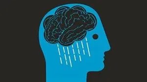
The pandemic's prolonged duration and uncertainty brought an immense emotional toll on the world, including FE exam candidates. Stress and anxiety relating to health concerns, economic insecurity, and social isolation affected many candidates' mental well-being, making it all the more difficult to focus on studying and preparing for the exam.

To combat anxiety and mental stress, it was important to have strong support systems in place. Family, friends, and peers played an integral role in providing emotional support and encouragement. Online communities emerged as a vital resource, offering a platform for candidates to connect, share experiences, and find solace in knowing they were not alone in facing these struggles.

 

Conclusion

The COVID-19 pandemic and global lockdown undoubtedly brought along many challenges for aspiring engineers preparing for the FE exam. Shifting to remote learning, disrupting study routines, limiting access to resources, isolating everyone, and postponing exams posed significant hurdles for everyone. Additionally, the emotional toll and mental health challenges further compounded the difficulties faced by future examinees. However, these obstacles were not faced without resistance.

Resilience and adaptability were highlighted in the face of adversity during COVID-19 and were nothing short of inspiring. Despite the setbacks, FE exam candidates were able to demonstrate determination and resourcefulness by embracing remote learning, seeking alternative study resources, and adjusting their preparation strategies for this new world. As we continue forward, it is crucial to recognize the hardships faced by FE exam candidates during the pandemic and provide the necessary support and resources to combat future hindrances that we may face in the future.

While the pandemic may have hurt FE exam candidates, it has also shown the strength of their spirit and their unwavering commitment as engineers. As the world gradually recovers from this crisis, let us celebrate the resilience of these aspiring engineers and support their journey towards a brighter and more promising future. Are you on the path to becoming a professional engineer? School of PE’s FE and PE exam courses are just what you need! Learn more about our comprehensive course options now!

About the Author: Khoa Tran

Khoa Tran is an electrical engineer working at the Los Angeles Department of Water and Power and is currently pursuing his master's in electrical Power from the University of Southern California. He is fluent in both Vietnamese and English and is interested in outdoor activities and exploring new things.

It All Adds Up: Mathematics on the FE Electrical Exam Pt. 2

Welcome back to our introduction to mathematics! Continuing from where we left off, we will explore calculus, ordinary differential equations, linear algebra, and vector analysis.

In this Blog,

1. Calculus

        a. Derivative

    b. Integral

2. Ordinary Differential Equation

3. Matrix Operations

4. Vector Analysis

    a. Vector Addition and Subtraction

    b. Vector Dot Product

    c. Vector Cross Product

Calculus

A. Derivative

The derivative of a function determines the immediate rate of change. Visually, it represents the slope depicted by the original function.

The basic rules of derivative include: derivative of sum, derivative of product, and derivative of quotient. The derivative of the sum is straightforward; you just need to take the derivative of each term. When it comes to multiplication, we have the product rule (Eqn 1).

dy/dx = u dv/dx + v du/dx      (1)

And the quotient rule (Eqn 2) to use for the division.

dy/dx = (v du/dx-u dv/dx)/v²    (2) 

The chain rule is a formula for finding the derivative of the composite of 2 functions. The chain rule helps to differentiate composite functions (find the derivative of a composite function). Generally, there is an “inside function” and an “outside function” that are both differentiable (Orloff, 2023).

(d[(f(u)])/dx = (d[f(u)]) /du  du/dx   (3) or 

f(g(x))' = f'(g(x))*g'(x)   (4)

B. Integral

The integral, or antiderivative, permits the calculation of the area under a curve or between curves.

Basic techniques for integrals:

1. Look for ways to simplify the integral with algebra before integrating.

2. Refer to the indefinite integrals on page 49 of the FE reference handbook.

3. Plug in the initial value and solve for the constant.

When integrals are more complicated, other methods of integration that can be used are:

1. Integration by Parts

2. Substitution

I. Integration by Parts

Integration by parts evaluates integrals of products of functions. It is based on the product rule of differentiation, which states that the derivative of the product of two functions is equal to the first function times the derivative of the second function, plus the second function times the derivative of the first function (Strang & Herman, 2022).

∫ u dv = uv - ∫ v du   (5) 

II. Substitution

U-substitution, also known as “Integration by Substitution” or “The Reverse Chain Rule”, is a method to simplify and evaluate integrals by use of substitution. To begin, ensure the integral is written in its standard form:

∫ f(g(x))g'(x) dx,   (6)

Then substitute in the variable “u.”

 ∫ f(u) du   (7) 

This replacement reduces a complicated expression into a simpler form that can be more easily evaluated.

The U-substitution is as follows (Mathematics LibreTexts, 2020):

1. Identify an expression within the integrand which appears to be a derivative of some function.

2. Choose a new variable "u" to represent the chosen expression. Do not forget to include the corresponding differential "du" to the derivative of "u" with respect to the original.

3. Rewrite the entire integral and substituting in the new variable "u", effectively replacing the complicated expression with "u".

4. Evaluate the new integral with respect to "u" using standard integration techniques, which may involve simpler rules or known integral formulas.

5. Finally, substitute the original variable back into the result by replacing "u" with the expression chosen in step 2.

Ordinary Differential Equation

A differential equation is a mathematical equation that involves an unknown function and its derivatives. It describes the relationship between the function and its rates of change. In essence, a differential equation expresses how the function's behavior changes based on its current state and the values of its derivatives (Herman, 2018).

The FE Reference Handbook provides a comprehensive collection of equation forms necessary for solving first-order and second-order homogeneous differential equations. These invaluable resources can be found on pages 52 and 53 of the handbook. To further enhance your understanding and proficiency, you can explore additional illustrative examples by following this link.

Matrix Operations

Matrix operations refer to various mathematical operations performed on matrices, which are rectangular arrays of numbers. Matrix operations allow for the manipulation, combination, and transformation of matrices, enabling the analysis of systems of linear equations, geometric transformations, and other mathematical applications.

In this section, I will not go too in-depth since you can use a calculator to manipulate matrices in the FE exam. You can visit this link to do matrix multiplication and this link on how to find the inverse and adjoint of a matrix.

Vector Analysis

A vector embodies the essence of a physical property, possessing not only its size but also its orientation. Its portrayal in three-dimensional space is accomplished by its x, y, and z constituents (Corral, 2023), often denoted as

F = a_x i + a_y j + a_z k   (8)

where:

a_x, a_y, a_z are the component magnitudes in the x, y, and z directions.

i,j,k are the unit vectors establishing coordinate direction for the vector.

The magnitude of vector F is calculated as:

F = √(〖a_x〗² +〖a_y〗² +〖a_z〗² )   (9)

A wide array of operations can be performed with vectors, benefiting from their linear nature, which ensures clear and precise outcomes.

Among the operations involving vectors are addition, subtraction, and multiplication, which are essentially akin to basic algebraic procedures. Scalar multiplication entails the multiplication of a scalar by a vector. The dot product, on the other hand, determines the angle between two vectors.

 

A. Vector Addition and Subtraction

Vector addition is the process of combining two or more vectors to obtain a resultant vector. Vector subtraction involves a reversal in direction, achieved by adding negative vectors. A negative vector possesses an equal magnitude to that of a positive addition vector but points in the opposite direction.

A ± B = (a_x ± b_x)i + (a_y ± b_y)j + (a_z ± b_z)k   (10)

B. Vector Dot Product

Also known as the scalar product, it is the operation that yields a scalar value by taking the sum of the products of the corresponding components of two vectors (Corral, 2023).

A∙B = (a_x b_x) + (a_y b_y) + (a_z b_z)   (11) (this produces a scalar)

or

A∙B = |A||B|cosθ = B∙A (12) (this produces the projection)

By rearranging the equation, the dot product can be utilized to ascertain the angle between two vectors, as illustrated in Figure 1. This rearrangement involves employing the cosine of the angle equation for the dot product.

cos θ = (A∙B) / |A||B|   (13)

Figure 1

C. Vector Cross Product

 The cross product yields a third vector, adhering to the principles of the right-hand rule, which resides orthogonal to the plane encompassing the initial two vectors. As vector A gracefully intertwines with vector B, it imparts the orientation of vector C, unfolding a trajectory perpendicular to their shared plane (Figure 2) (Corral, 2023).

Figure 2

The cross product is illustrated as a 3x3 matrix:

The sense of A X B is determined by the right-hand rule:

A × B = |A||B|n sin θ (14)

Where,

n is the unit vector perpendicular to the plane of A and B.

Conclusion

Although this blog provides an overview of mathematical topics found on the FE Electrical exam, you can find a more thorough explanation in School of PE’s FE Electrical exam review course. Learn more or register for a course now!

About the Author: Khoa Tran

Khoa Tran is an electrical engineer working at the Los Angeles Department of Water and Power and is currently pursuing his master's in electrical Power from the University of Southern California. He is fluent in both Vietnamese and English and is interested in outdoor activities and exploring new things.

It All Adds Up: Mathematics on the FE Electrical Exam

For those looking to take the Fundamentals of Engineering (FE) Electrical Engineering (EE) exam, we will delve into various concepts and components of mathematics, including:

 

1. Algebra and trigonometry

2. Complex numbers

3. Discrete mathematics

4. Analytic geometry

5. Calculus

6. Ordinary differential equation

7. Matrix Operation

8. Vector Analysis

Please note that the materials presented here are an overview. We encourage you to explore further resources if you wish to learn more about any particular topic.

In this blog,

1. Algebra and Trigonometry

    a. Algebra

    b. Trignometry

2. Complex Numbers

    a. Rectangular Form

    b. Polar Form

3. Discrete Mathematics

4. Analytic Geometry

    a. Slope of Equation

    b. Conic Section

Algebra and Trigonometry

A. Algebra

Algebra serves as an essential cornerstone in the realm of engineering. Nearly all analytical assessments in engineering require the use of algebraic equations. To adequately equip oneself for the FE Electrical exam, it is paramount to possess the proficiency to adeptly manipulate elementary algebraic equations, enabling the subsequent determination of solutions. This segment showcases illustrative instances of equation manipulations for comprehensive comprehension.

 

B. Trigonometry

Within the “Mathematic” section of the FE Reference Handbook, one can find a comprehensive compilation of essential trigonometric relations.

A notable use of trigonometry is analyzing the behavior of right triangles (Figure 1).

Figure 1

sin θ = y/r; cos θ = x/r; tan θ = y/x; cot θ = x/y; csc θ = r/y

sec θ = r/x

However, for non-right triangles, we cannot apply the above trigonometric relation to solve for the unknown values. Using the law of sines and cosines, all unknowns of a triangle can be characterized (Figure 2).

Figure 2

The law of sines is depicted below:

 a/sin A = b/sin B  = c/sin C

The law of cosines is depicted below:

a²= b²+ c² – 2bc cos A 

b²= a²+ c² – 2ac cos A
 

c²= a²+ b² – 2ab cos C

Complex Numbers

Complex numbers are a mathematical characterization equation that combines both a real part and an imaginary part (Electronics Tutorials, n.d.). It is typically written in the form

y = a + jb (1)

Where,

 a = real component

b = imaginary component, and j is the imaginary variable with the unit of √(-1). 

Complex numbers allow for the representation and manipulation of quantities that involve both real and imaginary components, extending the number system beyond the realm of real numbers.

There are two forms that the complex numbers can be represented: rectangular form or polar form (Electronics Tutorials, n.d.).

 

A. Rectangular Form

In the context of complex numbers, the rectangular form refers to a way of representing a complex number using its real and imaginary parts.

y = a + jb

B. Polar Form

In complex numbers, the polar form represents a way of expressing a complex number using its magnitude (or modulus) and argument (or angle). A complex number in polar form is written.

y = r(cos cos θ + jsin sin θ)=  z∠θ

To convert the complex number from rectangular form  to polar form, we can use the following formulas:

z = √(a²+b² )

θ = (b/a)  (in degree)

Conversely, to convert a complex number from polar form to rectangular form, we can use the following formulas:

a = r × cos cos θ 

b = r × sin sin θ 

Complex numbers can be added, subtracted, multiplied, and divided. Let’s say we have these 2 complex numbers:

A = 2+3j

B = -1+4j

Given the above values, complex numbers can be added and subtracted in rectangular form:

1. A + B = 2 + (-1) +3j  +4j  = 1 + 7j

2. A – B = 2 – (-1) + 3j - 4j = 3 - j

While, multiplying and dividing is performed in the polar form:

1. Convert the complex number A and B into polar form

a. For A: z = √(2²+3² ) = 3.6056 and θ = (3/2) = 56.31 deg . So, A = 3.6056 ∠56.31deg.

b. For B: z = √(〖(-1)〗²+4² ) = 4.123 and θ = (4/(-1)) =104.04 deg . So, B = 4.123∠104.04deg.

2. When A x B:

A x B = 3.6056∠56.31deg × 4.123∠104.04deg = = 3.6056*4.123∠(56.31+104.04) =14.87∠160.35deg

3. When A / B: 

A / B = (3.6056∠56.31) / (4.123∠104.04) = 3.6056/4.123∠(56.31-104.04) = 0.87∠-47.73deg. 

Discrete Mathematics

Discrete mathematics is a branch of mathematics that deals with mathematical structures and techniques focused on countable or finite sets. It encompasses topics such as graph theory, combinatorics, set theory, logic, and algorithms, which are instrumental in solving problems involving discrete structures and countable sets (Hayes et al., n.d.).

Set theory is key within discrete mathematics, it is the study of collections of objects. Set operations, such as union (∪), intersection (∩) , and complement (') are fundamental in set theory (Hayes et al., n.d.).

Example:

Suppose we have two sets A = {1, 2, 3} and B = {2, 3, 4}. The union of A and B (A ∪ B) is then represented as {1, 2, 3, 4}, and all the distinct elements from both sets are outputted. The intersection of sets A and B (A ∩ B) is then represented as {2, 3}, and all the common elements between the sets are outputted. The complement of set A (A') is the set of all elements not present in A.

For further information about discrete mathematics, you can visit this website to explore more!

Analytic Geometry

Analytic geometry, also known as coordinate geometry, is a branch of mathematics that combines algebraic techniques with geometric concepts. It involves studying geometric figures and relationships using algebraic equations and coordinates.

In analytic geometry, points, lines, curves, and other geometric objects are shown using coordinates in a coordinate system: Cartesian coordinate system. The Cartesian coordinate system consists of two perpendicular lines called the x-axis and y-axis, intersecting at a point called the origin (Nykamp, n.d.). Each point in the plane is uniquely identified by its x-coordinate (horizontal position) and y-coordinate (vertical position).

A. Slope of Equation

The x-y plane serves as a two-dimensional coordinate system that represents pairs of values (x, y). These pairs, known as ordered pairs, are referred to as points. A line can be defined by two points. The equation of a line can be expressed in the slope-intercept form, which is given by:

y = mx+b

Where,

m is the slope of the line

 b = y intercept, where b is the value of y when  x = 0;

The slope between two points can be found by:

m=(y₂-y₁)/(x₂-x₁ ) 

By rearranging the slope equation, it becomes possible to calculate the value of "b" using any point that is provided on the line.

b = y - mx

Example:

Given two points (10, 20) and (-30, -40). Find the line equation

1. m = (-40-20) / (-30-10) = (-60) / (-40) = 1.5

2. We will pick the first point (10, 20) to solve for b

b = y - mx = 20 – (1.5)(10) = 5

Therefore,  y =1.5x + 5

B. Conic Section

Conic sections are an important class of equations involving two variables. They encompass four types: parabolas, ellipses, hyperbolas, and circles. The term "conic section" originates from the concept of intersecting a cone with a plane in different configurations.

Figure 3

When a plane intersects a three-dimensional double right circular cone at various positions and angles, it gives rise to conic sections (refer to Figure 3). The equation describing the resulting conic section depends on the characteristics of the cone, specifically the angle between the cone's side and its axis (ϕ), as well as the angle between the intersecting plane and the cone's axis (θ). The relationship between the plane and the cone is quantified by the eccentricity (e) (Strang & Herman, 2022).

In the FE exam, the problems pertaining to this section are presented in a straightforward manner. One can employ the provided equations and relationships to determine the unknown values based on the specific type of conic section involved. It is crucial to thoroughly read and comprehend the problem statement in order to correctly identify and utilize the appropriate equation.

Conclusion

This is a lot of information to sort through on first reading, so please take the time to reread and practice the problems on your own. We will finish the other half in the second part of this blog. Are you interested in a comprehensive exam review course that will cover the topics of this blog and more? Check out School of PE’s FE Electrical exam review courses now.

References

Electronics Tutorials. (n.d.). Complex Numbers and Phasors in Polar and Rectangular Form. Electronics Tutorials. Retrieved July 6, 2023, from https://www.electronics-tutorials.ws/accircuits/complex-numbers.html

Hayes, A., Parvej, M. R., Vee, H. Z., Nelson, A., & Khim, J. (n.d.). Discrete Mathematics. Brilliant. Retrieved July 5, 2023, from https://brilliant.org/wiki/discrete-mathematics/

Nykamp, D. Q. (n.d.). Cartesian coordinates. Math Insight. Retrieved July 6, 2023, from https://mathinsight.org/cartesian_coordinates

Strang, G., & Herman, E. '. (2022, September 7). 11.5: Conic Sections. Mathematics LibreTexts. Retrieved July 6, 2023, from https://math.libretexts.org/Bookshelves/Calculus/Calculus_(OpenStax)/11%3A_Parametric_Equations_and_Polar_Coordinates/11.05%3A_Conic_Sections

About the Author: Khoa Tran

Khoa Tran is an electrical engineer working at the Los Angeles Department of Water and Power and is currently pursuing his master's in electrical Power from the University of Southern California. He is fluent in both Vietnamese and English and is interested in outdoor activities and exploring new things.

Cracking Control Systems: What You Need to Know for the FE Electrical Exam

Ever wonder how auto-pilot works or how assembly robots move so quickly yet accurately? Control Systems. Not only does this apply to automation or specialized industries but also to our refrigerators, our cars, and everything where a device or system needs to have a desired output, control systems are implemented.

The FE requires examinees to understand and be able to solve questions regarding control systems. In this blog, we will go over a brief overview of what control systems are and what equations are expected for test takers to know for the exam.

In this Blog,

1. What are Control Systems?

2. Stability Theorem

3. Coefficient Test

4. Routh-Hurwitz Criterion

What are Control Systems?

A control system is a system of devices that regulates the different behaviors of other devices to achieve a desired result. There are two types of control loops: open-loop and closed-loop.

Open-loop control systems have the control action totally independent of the outcome of their systems. A simple example of this is an electric hand dryer; the hot air (output) remains on for as long as an object is detected under its sensor (input), regardless of how dry the object may be.

Closed-loop control systems, on the other hand, have the input affected by the output in order to achieve the desired output. This behavior is referred to as feedback. To bring back a previous comparison, refrigerators are an example of a closed-loop system, where the cooling devices have their output throttled to maintain a certain temperature inside the refrigerator. This not only ensures that the temperature in the device is constant but also a balance between cooling time and power efficiency.

Control system stability refers to the behavior of a system over time and its ability to maintain a desired state or equilibrium. A stable control system is one that, after experiencing a disturbance or change, eventually returns to its original state or reaches a new stable state.

In the Stability section of the Control System topic for the Fundamental of Engineering (FE) exam, there are two methods to determine the stability of the system:

1.Stability Theorem

2.Coefficient Test

3.Routh-Hurwitz Criterion

Stability Theorem

We can use the Stability Theorem to determine the system’s stability.

1.Stable System: A system is considered stable when the poles of its transfer function reside on the left side of the s-plane. However, if the poles move closer to the origin, the system’s stability decreases (Stefani, 2002, 71).

Ex: H (s) = 2 / ((s+1) (s+2))

a. Set the denominator equal to zero, we have s = -1 and s = -2 We know the poles lie on the left-hand side of the s-plane. Therefore, the system is stable.

Figure 1

2. Marginally Stable System: A system is considered marginally stable when the poles are present in the imaginary axis (Stefani, 2002, 71).

Ex: H (s) = 2/ (s²+2) = 2/((s+√2 i) (s-√2 i))

a. Set the denominator equal to zero, we have s = ±√2 i. We know the poles lie on the imaginary axis of the s-plane. Therefore, the system is marginally stable.

Figure 2

3. Unstable System: A system is considered unstable when there are repeated poles on the imaginary axis of the s-plane and/or poles in the right half of the s-plane (Stefani, 2002, 71).

Ex: H(s) = 2 / (〖(s〗²+2) (s-1)) = 2 / ((s+√2 i)(s-√2 i)(s-1))

a. Set the denominator equal to zero, we have s = ±√2 i  and s = 1. We know the poles lie on the imaginary axis of the s-plane. But there is a pole on the right-hand plane. Therefore, the system is unstable.

Figure 3

Coefficient Test

For a high-order polynomials transfer function, if there is a missing s term, it is safe to say that the system is unstable (Stefani, 2002, 144-145).

Example, a transfer function T(s) = 6s⁵ + 5s⁴ + 3s² + 7s + 10. The transfer function is missing the s³ term.

Routh-Hurwitz Criterion

The Routh-Hurwitz stability criterion is a mathematical method used to determine the stability of a linear control system. It provides a systematic approach to analyze the stability of a system by examining the coefficients of its characteristic equation.

The characteristic equation of a linear control system is obtained by setting the denominator of its transfer function equal to zero (Eqn. 1). It is typically a polynomial equation in terms of the system's parameters. The Routh-Hurwitz criterion uses the coefficients of the characteristic equation to construct a table called the Routh array or Routh table. The Routh array organizes the coefficients into rows and columns, allowing for a systematic evaluation of stability (Stefani, 2002, 145).

a_n sⁿ + a_(n-1) s^(n-1) + a_(n-2) s^(n-2) + ... + a₀ = 0 (1)

Arrange all the coefficients into the table below:

Table 1

sn	an	an-2	an-4
sn-1	an-1	an-3	an-5
sn-2	b1	b2	b3
sn-3	c1	c2	c3
:
s0

b₁ = (a_(n-1) a_(n-2) - a_n a_(n-3)) / a_(n-1)  (2)

b₂ = (a_(n-1) a_(n-4) - a_n a_(n-5)) / a_(n-1)  (3)

c₁ = (b₁ a_(n-3) - b₂ a_(n-1)) / b₁  (4)

c₂ = (b₁ a_(n-5) - b₃ a_(n-1)) / b₁  (5)

When all the coefficients a_n , a_n-1 , b₁ , c₁ are all of the same positive sign, and none is zero ,then the system is stable. Else, the system is unstable.

Let’s examine this T(s) transfer function stability:

T(s) = s⁴ + 2s³ + 6s² + 4s + 1  (6)

Table 2

s4	1	6	1
s3	2	4
s2	b1	b2
s1	c1
s0	d1

b₁ = 2(6) - 4(1) / 2 = 4

b₂ = 2(1) - 1(0) / 2 = 1

c₁ = b₁(4) -2(b₂) / b₁ = 4(4) - 2(1)  /4 = 3.5

d₁ = c₁(b₂) - b₁(0) / c₁ = 3.5(1)- 4(0) / 3.5 = 1

Therefore, the complete table is:

Table 3

s4	1	6	1
s3	2	4
s2	4	1
s1	3.5
s0	1

By looking at the highlighted region, there is no change in sign, and all coefficients are positive. Therefore, the system is stable.

The quantity of right half-plane (RHP) roots in T(s) corresponds to the count of sign changes in the elements of the leftmost column of the array, progressing from the top to the bottom (Stefani, 2002, 147). We will change the value sign of s₁ value row in Table 3 to demonstrate this aspect.

Table 4

s4	1	6	1
s3	2	4
s2	4	1
s1	-3.5
s0	1

From Table 4, there are two signs of changes in the highlighted column (4 to -3.5 and -3.5 to 1); therefore, T(s) has two RHP roots.

Conclusion

We’ve gone over what control systems are and how to use the Stability Theorem, Coefficient Test, and Routh-Hurwitz Criterion, but for a more thorough and comprehensive study plan, I recommend checking out School of PE’s FE Electrical exam review course, which offers an extensive and detailed curriculum to ensure a comprehensive understanding of the subject matter. Good luck!

References

Stefani, R. T. (2002). Design of Feedback Control Systems. Oxford University Press.

About the Author: Khoa Tran

Khoa Tran is an electrical engineer working at the Los Angeles Department of Water and Power and is currently pursuing his master's in electrical Power from the University of Southern California. He is fluent in both Vietnamese and English and is interested in outdoor activities and exploring new things.